What previous days’ weather affected today’s weather? Historically, which states’ votes affected the outcome of different presidential elections? How does a single trade affect the price of a stock?
Modelling the weather, politics, and economics would be a very difficult task but we can explore questions like this in less complex mathematical systems such as the delayed Henon map [1]. The delayed Henon map is a time-delayed system represented by following equation,
Since it has an adjustable d parameter, which represents what dimension the function can be embedded in and provides us with a knob to turn to explore high dimensional dynamics. We can explore many different features about this map, the correlation dimension, fractal dimension, Lyapunov exponents, and much more but our primary focus will be looking at the sensitivities for this map. If you are interested in more information about this map, please consult Sprott 2005, a full reference is below. For the rest of this post, I will be using d=4. As we will see, this is more than adequate for the analysis I will show, but one could easily use d = 1456 if they wanted to. Due to the linearity of , a different choice of d will arrive at almost the same results.
So, how are the three questions posed above tied together? They all attempt to answer a common question. What is the sensitivity of each time lag in a function of the system [2]?
For the delayed Henon map, this would be akin to asking, how does affect
. We can infer this by taking the partial derivative of
with respect to each time lag. Using a partial derivative is like asking, if I vary
just slightly, how will
change. For the obviously non-zero time lags that would be,
To accurately determine how much the output of the function varies when each time lag is perturbed, we need to find the mean of the absolute values of the partial derivatives around the attractor. Thus we have,
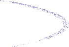
Since the delayed Henon map has a chaotic attractor and the values of vary, you can estimate the value of the sensitivities for 10,000 iterations of the time series. Initializing the map with a vector such as [.1, .1, .1, .1], we get the following strange attractor (with the first 1,000 iterations removed),

Delayed Henon Map with 9,000 points (d=4)
We arrive at the following sensitivities for d=4,
By estimating a system’s sensitivities, we can determine what is known as the lag space [3]. Dimensions with non-zero sensitivities make up this space and the largest dimension with a non-zero sensitivity also determines the embedding dimension. As we will see in another post, a neural network method can be devised to find the lag space of various time series.
References:
- Sprott JC. High-dimensional dynamics in the delayed Hénon map. Electron J Theory Phys 2006; 3:19–35.
- Maus A. and Sprott JC. Neural network method for determining embedding dimension of a time series. Comm Nonlinear Science and Numerical Sim 2011; 16:3294-3302.
- Goutte C. Lag space estimation in time series modelling. In: Werner B, editor. IEEE International Conference on Acoustics, Speech, and SignalProcessing, Munich, 1997, p. 3313.
This post is part of a series:
- Delayed Henon Map Sensitivities
- Inverted Delayed Henon Map
- Modeling Sensitivity using Neural Networks