Lyapunov spectra of inverted discrete dynamical systems

One can estimate the Lyapunov spectrum of dynamical systems and their inverted counterparts using local Jacobian matrices and Wolf’s algorithm. Basically, Jacobian matrices are calculated at each point in a trajectory and multiplied together to form a product matrix whose eigenvalues represent the Lyapunov exponents for the system studied. More specifically, these exponents measure the divergence of a ball of initial conditions as they move around an attractor, in this case, a strange attractor. As the Jacobians are multiplied together, Gram-Schmidt reorthonormalization is used to maintain the system of coordinates and unify the divergence because the ball of initial conditions quickly becomes an ellipisoid.

In 1985, Alan Wolf et al. published the paper that outlined a program that can be used to determine the spectrum of Lyapunov exponents for system’s whose equations are known. Wolf’s algorithm requires that the equations are linearized. After performing the necessary calculations, one can plug them into the program available here (in Python) and estimate the Lyapunov spectrum.

Here is an example of how to linearize the Henon map and more complex Tinkerbell map:

The Henon map:

$x_{t}%20=1-1.4x_{t-1}^2%2b.3y_{t-1}$

$y_{t}%20=x_{t-1}$

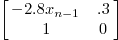
The Henon’s Jacobian matrix:

$\left[\matrix{-2.8x_{n-1}%26.3\cr%201%260}\right]$ Linearizing the Henon map:

$\left[\matrix{\partial%20x_{n}\cr\partial%20y_{n}}\right]=\left[\matrix{-2.8x_{n-1}%26.3\cr%201%260}\right]\left[\matrix{\partial%20x_{n-1}\cr\partial%20y_{n-1}}\right]$

Partial Code for Wolf’s algorithm:

def Henon(x, xnew, n):
	a=1.4
	b=0.3
	#   Nonlinear Henon map equations:
	xnew[1] = 1-a*x[1]*x[1]+b*x[2]
	xnew[2] = x[1]
	#   Linearized Henon map equations:
	xnew[3] = -2*a*x[1]*x[3]+b*x[5]
	xnew[4] = -2*a*x[1]*x[4]+b*x[6]
	xnew[5] = x[3]
	xnew[6] = x[4]
	return [x, xnew]

The Tinkerbell map:

$x_{n}=x_{n-1}^2-y_{n-1}^2%2b0.9x_{n-1}-0.6y_{n-1}$
$y_{n}=2x_{n-1}y_{n-1}%2b2.0x_{n-1}%2b0.5y_{n-1}$

The Tinkerbell’s Jacobian matrix:

$\left[\matrix{2x_{n-1}%2b0.9%26-2y_{n-1}-0.6\cr2y_{n-1}%2b2%262x_{n-1}%2b0.5}\right]$

Linearizing the Tinkerbell map:

$\left[\matrix{\partial%20x_{n}\cr\partial%20y_{n}}\right]=\left[\matrix{2x_{n-1}%2b0.9%26-2y_{n-1}-0.6\cr2y_{n-1}%2b2%262x_{n-1}%2b0.5}\right]\left[\matrix{\partial%20x_{n-1}\cr\partial%20y_{n-1}}\right]$

Partial Code for Wolf’s algorithm:

def tinkerbell(x, xnew, n):
	a =  0.9
	b = -0.6
	c =  2.0
	d =  0.5
	# Nonlinear
	xnew[1] = x[1]**2 - x[2]**2 + a*x[1] + b*x[2]   # x
	xnew[2] = 2*x[1]*x[2] + c * x[1] + d * x[2]	 # y
	# Linearized
	xnew[3] = 2 * x[1] * x[3] + a * x[3] - 2 * x[2] * x[5] + b * x[5] # delta x
	xnew[4] = 2 * x[1] * x[4] + a * x[4] - 2 * x[2] * x[6] + b * x[6] # delta x
	xnew[5] = 2 * x[2] * x[3] + c * x[3] + 2 * x[1] * x[5] + d * x[5] # delta y
	xnew[6] = 2 * x[2] * x[4] + c * x[4] + 2 * x[1] * x[6] + d * x[6] # delta y
	return [x, xnew]

To estimate the Lyapunov spectrum of the inverted system. One can simply reverse the signs on the exponent values of the forward system or take the more roundabout way and estimate them using Wolf’s algorithm.

To estimate the exponents, it is necessay to obtain to invert the system’s equations. In some cases, this is not possible such as the case of the Logistic map where each point could come from one of two previous points. To estimate the inverted system’s Jacobians (and the inverted system’s equations), one can simply invert the Jacobian matrix of the forward equations.

For the Henon map:

$\frac{1}{0-0.3}\left[\matrix{0%26-0.3\cr%20-1%26-2.8x_{n-1}}\right]$

For the Tinkerbell map (and those with a magnifying glass):

$\frac{1}{(2x_{n-1}%2b0.5)(2x_{n-1}%2b0.9)-(2y_{n-1}%2b0.6)(-2y_{n-1}-2)}\left[\matrix{2x_{n-1}%2b0.5%262y_{n-1}%2b0.6\cr-2y_{n-1}-2%262x_{n-1}%2b0.9}\right]$

The last issue that needs to be solved is generating data for the system. Since the system is inverted, the system has most likely turned from an attractor to a repellor and thus any trajectory will wander off to infinity. Therefore, we use the forward system’s equations and use the linearizations for the inverted system to estimate the Lyapunov spectrum. You can use the following Python program and plug in the code above to see an example.