Similar to Neural Networks, Support Vector Machines (SVM) are powerful modelling techniques in machine learning that can be applied to a variety of tasks. SVMs are primarily used to classify data while one of its variants, Support Vector Regression (SVR), can be used for time series analysis. In this post, we will perform SVR on chaotic time series using common Python libraries and a simple wrapper program.
The following libraries will be required to use the script I will demonstrate using Python 2.7:
- Numpy
- Scipy
- Scikits.Learn (a toolbox that hosts a variety of machine learning algorithms and requires Numpy and Scipy)
- MatPlotLib (used for graphing and visualization)
- Other libraries such as SetupTools may be required depending on your system
You can download these from their websites or if you are using Windows “Unofficial Windows Binaries for Python Extension Packages”
With the packages installed, we can begin to build a program that fits an SVR model to chaotic data. First, we define a time series. In this case, I will use the Delayed Henon Map with a delay of 4, for more information please see my posts on that system.
The model will be embedded in a d dimension space.
def TimeSeries(cmax, transient, d):
  return DelayedHenon(cmax, transient, d)
def DelayedHenon(cmax, transient, d):
  temp = []
  rF = [] # Features
  rT = [] # Targets
  dX = []
  i = 0
  while i < d:
    dX.append(0.1)
    i = i + 1
  while i <= cmax + transient:
    x = 1 - 1.6 * dX[i-1] ** 2 + 0.1 * dX[i-4]
    if i > transient-d:
      temp.append(x)
    if i > transient:
      rT.append(x)
    dX.append(x)
    i = i + 1
  rF = SlidingWindow(temp, d)
  return {"F":rF, "T":rT}
I added a function that formats the data properly so it can be used by the SVR Fit function:
def SlidingWindow(x, d):
  i = d
  y = []
  while i < len(x):
    temp = []
    j = 1
    while j <= d:
      temp.append(x[i - d + j])
      j = j + 1
    y.append(temp)
    i = i + 1
  return y
We then define the model, note that SVR has a few user defined parameters which can be chosen to fit the data better.
clf = svm.SVR(kernel='rbf', degree=d, tol=tolerance, gamma=gam, C=c, epsilon=eps)
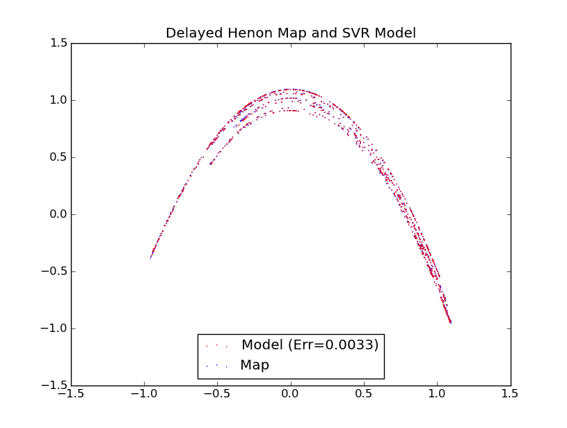
In this case, you can choose the following parameters to produce a model with an error near 0.0035 for 1024 points taken from the time series. In practice, you can create a training algorithm to find these values.
  gam = 0.117835847192
  c = 1.02352954164
  eps = 0.00163811344978
  tolerance = 0.00539604526663
  d = 5
  cmax = 1024
Finally, we create functions to fit the time series and plot the results:
def Fit(cmax, d, tolerance, gam, c, eps):
  data = TimeSeries(cmax, random.randint(0,10000), d)
  test = TimeSeries(cmax, random.randint(0,10000), d)

  x = data["F"]
  y = data["T"]

  sout = test["T"]

  clf = svm.SVR(kernel='rbf', degree=d, tol=tolerance, gamma=gam, C=c, epsilon=eps)

  try:
    m = clf.fit(x, y)
  except:
    return [1000, clf, sout, sout]

  mout = clf.predict(test["F"])

  # Determine the error for the system
  err = 0
  i = 0
  while i < len(mout):
    err += (mout[i] - sout[i])**2
    i = i + 1
  err = math.sqrt(err / (len(mout)+.0))

  return [err, clf, mout, sout]

def Plotter(err, mout, sout, SaveGraph):
  plt.title("SVR: Err=" + str(err))
  plt.scatter(sout[0:len(sout)-2], sout[1:len(sout)-1], s=1, marker='o', edgecolors='none')
  plt.scatter(mout[0:len(mout)-2], mout[1:len(mout)-1], s=1, marker='o', edgecolors='none', facecolor='r')

  plt.show()
  if SaveGraph:
    try:
      plt.savefig("svr")
    except:
      # Do Nothing
      SaveGraph = SaveGraph
  plt.clf()
Here is the final program after putting all of the functions together (and moving some stuff around) with example output:
#!/usr/bin/env python
from scikits.learn import svm
import random
import math
import matplotlib.pyplot as plt

d = 5       # Degree of the SVR model
cmax = 1024 # Number of points to run

def TimeSeries(cmax, transient, d):
  return DelayedHenon(cmax, transient, d)

def main():
  global cmax, d, perturbation
  gam = 0.117835847192
  c = 1.02352954164
  eps = 0.00163811344978
  tolerance = 0.00539604526663
  # Create and Fit a model to data, we just need to create support vectors
  [err, svr, mout, sout] = Fit(cmax, d, tolerance, gam, c, eps)
  Plotter(err, mout, sout, False)
  print "error: ", err
def DelayedHenon(cmax, transient, d):
  temp = []
  rF = [] # Features
  rT = [] # Targets
  dX = []
  i = 0
  while i < d:
    dX.append(0.1)
    i = i + 1
  while i <= cmax + transient:
    x = 1 - 1.6 * dX[i-1] ** 2 + 0.1 * dX[i-4]
    if i > transient-d:
      temp.append(x)
    if i > transient:
      rT.append(x)
    dX.append(x)
    i = i + 1
  rF = SlidingWindow(temp, d)
  return {"F":rF, "T":rT}
def Fit(cmax, d, tolerance, gam, c, eps):
  data = TimeSeries(cmax, random.randint(0,10000), d)
  test = TimeSeries(cmax, random.randint(0,10000), d)

  x = data["F"]
  y = data["T"]

  sout = test["T"]

  clf = svm.SVR(kernel='rbf', degree=d, tol=tolerance, gamma=gam, C=c, epsilon=eps)

  try:
    m = clf.fit(x, y)
  except:
    return [1000, clf, sout, sout]

  mout = clf.predict(test["F"])

  # Determine the error for the system
  err = 0
  i = 0
  while i < len(mout):
    err += (mout[i] - sout[i])**2
    i = i + 1
  err = math.sqrt(err / (len(mout)+.0))

  return [err, clf, mout, sout]

def Plotter(err, mout, sout, SaveGraph):
  plt.title("Delayed Henon Map and SVR Model")
  p1 = plt.scatter(sout[0:len(sout)-2], sout[1:len(sout)-1], s=1, marker='o', edgecolors='none')
  p2 = plt.scatter(mout[0:len(mout)-2], mout[1:len(mout)-1], s=1, marker='o', edgecolors='none', facecolor='r')
  plt.legend([p2, p1], ["Model (Err="+ str(round(err,4))+")", "Map"], loc=8)

  plt.draw()
  plt.show()
  if SaveGraph:
    try:
      plt.savefig("svr")
    except:
      # Do Nothing
      SaveGraph = SaveGraph
  plt.clf()

def SlidingWindow(x, d):
  i = d
  y = []
  while i < len(x):
    temp = []
    j = 1
    while j <= d:
      temp.append(x[i - d + j])
      j = j + 1
    y.append(temp)
    i = i + 1
  return y

def WriteFile(err, BestTol, BestGam, BestC, BestEps, s):
  # Write the model, sensitivities to a file
  f = open("sensitivities", "w")
  f.write("Model Parameters:\n")
  f.write("d=" + str(d) + "\n")
  f.write("gam=" + str(BestGam) + "\n")
  f.write("c=" + str(BestC) + "\n")
  f.write("eps=" + str(BestEps) + "\n")
  f.write("tolerance=" + str(BestTol) + "\n")
  f.write("Model Data:\n")
  f.write("err=" + str(err) + "\n")
  f.write("s=" + str(s) + "\n")
  f.close()
main()
Example Output:
err: 0.00381722720161

To fit data taken from other systems, simply change the Timeseries function.
Comments
2 responses to “Modelling Chaotic Systems using Support Vector Regression and Python”