This will start a series on the Particle Swarm Optimization algorithm.
The following topics will be covered:
- An overview of Particle Swarm Optimization Algorithm
- In-depth details of the algorithm
- More applications of Particle Swarm Optimization
Particle Swarm Optimization (PSO)
This algorithm is often used to optimize functions in rather unfriendly non-convex, non-continuous search spaces. The idea behind the algorithm involves a swarm of particles flying through a space both collaboratively and independently.
Instead of talking about particles, it is helpful to imagine that the swarm of particles is actually a flock of birds flying through a mountain range. Their goal is to find the best nesting site within this ‘search space’. The ideal nesting site has few predators, plenty of food sources, and many resources for building sturdy nests. Instead of the continuous motion that we often see in flying birds, each of the birds updates where it is going to head and how fast after each ‘turn’. So each of the birds makes a decision based on the birds around them and then they all move at the same time. This is repeated until some sort of stopping criterion has been satisfied (or the best nesting location has been found).
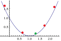
The following set of illustrations show how a swarm could find the minimum of a parabola.
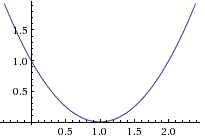
We randomly place 5 particles within the search region. The best performing particle so far is seen in green at about 1.25.
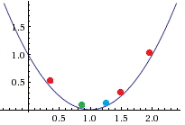 All of the particle look at their own position and their neighbors and update their positions and velocities. Often they end up moving towards the best performing particle from the previous step (now seen in blue). The new best performing particle (in green) is close to 0.85.
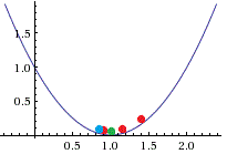 With the next update, the particles start converging to the same positions and overlap slightly. The new best particle is close to 1.0.
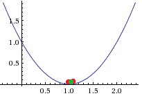 Almost all of the particles converge to the correct answer in this step. However, further iterations may be necessary to determine if the correction minimum has been achieved.
How is this useful?
We can extend this example to high dimensional spaces such as a 100 dimensional paraboloid. Or the weight space for a neural network where each particle becomes a neural network that is looking for the best way to fit a set of data. Other examples could include Support Vector Machines or even the optimal choice of crops for a growing season. The applications are nearly endless.
In the next section, we will go over how the algorithm actually works and an example involving the optimization of a function.
This post is part of a series:
- An overview of Particle Swarm Optimization Algorithm
- In-depth details of the algorithm
- More applications of Particle Swarm Optimization


Comments
3 responses to “An Overview of Particle Swarm Optimization”