In-depth details of Particle Swarm Optimization

In the first part of this series on Particle Swarm Optimization (PSO), I posted an general overview of the algorithm and an example of how the algorithm searches for the minimum of a parabola. In this post, I explain an example of the algorithm constructed in Python. I will end with an example problem, called the Rastrigin function, a function that researchers use to test their optimization algorithms on.

The full Python code that I will be discussing is located here. It may be helpful to open this code since I will only be discussing specific portions of the code. If you want to run the code, please save the page as a .py (Python) file.

The file is set up in the following way:
– global variables and user-defined parameters
– function F(): the function being optimized, in the example file, I use the Rastrigin function
– function main(): the function that constructs the swarm and attempts to optimize F
– class Particle: the functions and local variables associated with each Particle

The function main, constructs the swarm and iterates for a user-defined number of trials (cmax). The best velocity, position, and error are saved and output at the end of the program. It is not necessary to use the number of trials to signal the end of optimization. One could also stop the optimization if the best error achieves a certain value or if all of the particles are below some error bound.

During optimization, particles’ behavior are determined by the following set of equations:

The first equation v_ij(t) determines the velocity of particle i in dimension j for time step t. Particles adjust their trajectory in the search space according to their local neighborhood’s best position x**, their own best position x*, and their previous velocity. The first term of the velocity characterizes how much the previous velocity affects the new velocity with w set to 1 in the code. In the code, a dampening parameter is included that can be used to slow particles as optimization progresses. The second term or “cognitive” term with c₁r₁ pull particles back to their best previous position. The third term or “social” term with c₂r₂ pushes particles together so they fly collaboratively through space. The second equation x_ij(t) determines the position of particle i in dimension j for time step t. New positions are determined by the previous position and the current velocity.

In the Python code, the particle class randomly initializes the positions and velocities (the InitPosition(self) and InitVelocity(self) functions) for each particle within some search space. After each time step in the optimization, the UpdateVelocity(self) and UpdatePosition(self) functions are called to construct new velocity and position vectors for each particle.

Within the main function, the particles’ positions are evaluated after each update as the swarm moves towards the optimal position in the space.

The following graphs are from an example trial of the algorithm run on the 1-D Rastrigin function:

PSO variations are often tested on the Rastrigin function because of how simple changes to the parameter d can extend the function to higher dimensions. Additionally, the number of deep local optima is quite large, as seen in the graph below. The global optimum is at x=0. For these results, the following parameters were used:

# The dimension of the function
num_dimensions = 1
# The number of particles in the swarm
num_particles = 5

# Bounds on the positions and velocities
v_max = 5
v_min = -5
p_min = -10
p_max = 10
# The number of updates to do
cmax = 1000
# The amount to dampen the velocity after each update
dampener = 1
dampen_rate = 1

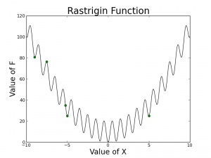
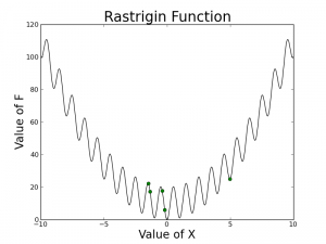
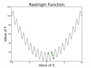
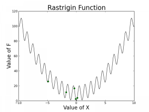
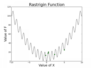
As you can see, the swarm does not necessarily converge to the global optimum (x = 0) but they are all somewhat close. If you measured the best position, at least one particle has encountered the optimal position during optimization but the particle did not end up settling down because of how the parameters, the dampening factor, w, c₁, and c₂ were chosen. One of the simplest ways to improve the algorithm is to allowing the velocity to decay (w < 1 or dampening factor) which should help all of the particles converge to an optimum.

Of course, this is just one example of how to set up the algorithm. Many researchers have experimented with portions of the algorithm trying to find the best way to optimize a function. As we will see later, changes to the particle’s equations and the distributions used to select r₁ and r₂ are just a few open problems in PSO.

This post is part of a series:

1. An overview of Particle Swarm Optimization Algorithm
2. In-depth details of the algorithm
3. More applications of Particle Swarm Optimization